LAZ to classified point cloud: every processing step explained

Jul 13, 20268 MIN READWorkflow

Hillshaded bare-earth digital terrain model derived from airborne LiDAR, showing hillfort earthworks and field boundaries with vegetation and structures filtered out. — A digital terrain model: the end of the chain, not the classified cloud it was derived from. Source: data.gov.uk, Open Government Licence v3.0.

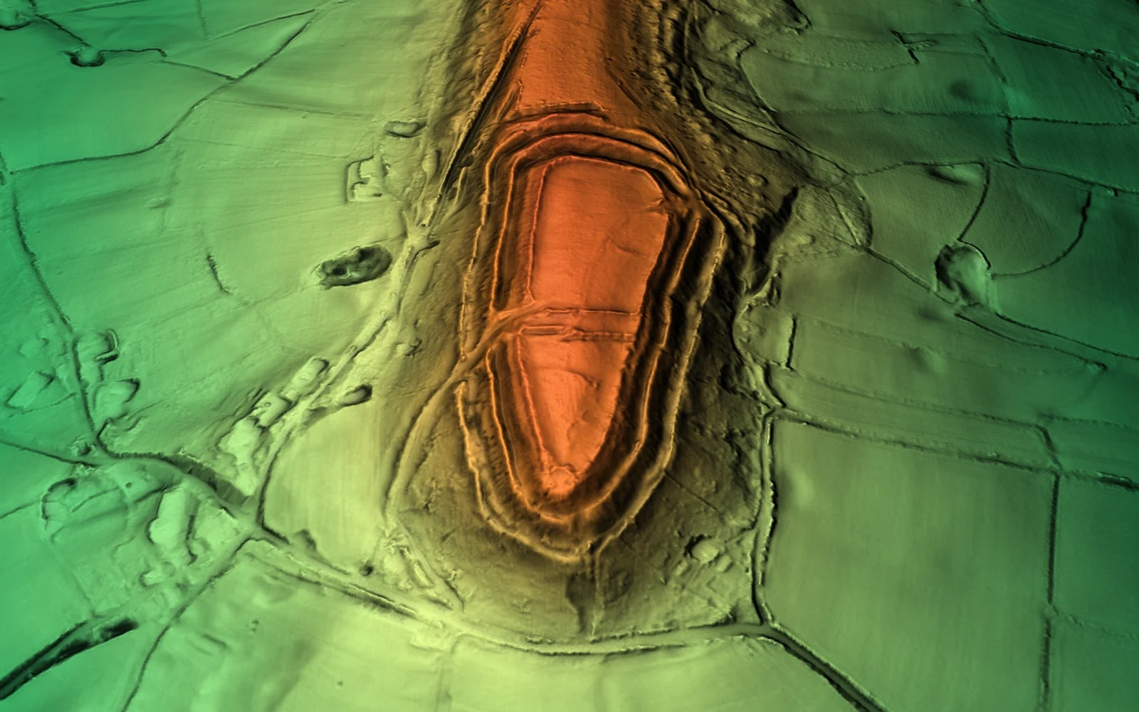
A point cloud is a set of points that represents a 3D scene. Before an AI model can label those points, the team must check the delivered LAZ file and prepare it for the model.

This post follows the path from a LAZ file to a checked classified point cloud.

1. Read the LAZ file

LAZ is a lossless compressed form of the LAS point-cloud format. Decompression restores the coordinates and stored point attributes [1].

Start with the file header. Check the point count. Then check the spatial bounds and point-record format. Read the points and confirm that the count and extent match.

Keep the attributes that later steps need. These can include return information and a flight-line identifier for strip checks [1], [2].

2. Check the coordinate system

The horizontal reference places points on the map. The vertical reference defines what their elevations mean.

Airborne LiDAR combines scanner measurements with the aircraft trajectory. A wrong transformation can change mapped distances or elevations [3].

Check the declared reference system and units. Then compare the cloud with independent control. Correct metadata does not prove that the coordinate transformation worked correctly.

3. Align overlapping flight strips

Airborne surveys usually contain overlapping flight strips. An error can leave one strip slightly offset from the next [4].

The overlap makes the error visible. One roof can appear as two nearby surfaces instead of one.

Strip adjustment compares matching surfaces and estimates a correction. Glira and colleagues tested this type of method across 103 strips. Their study does not set a tolerance for every project [4].

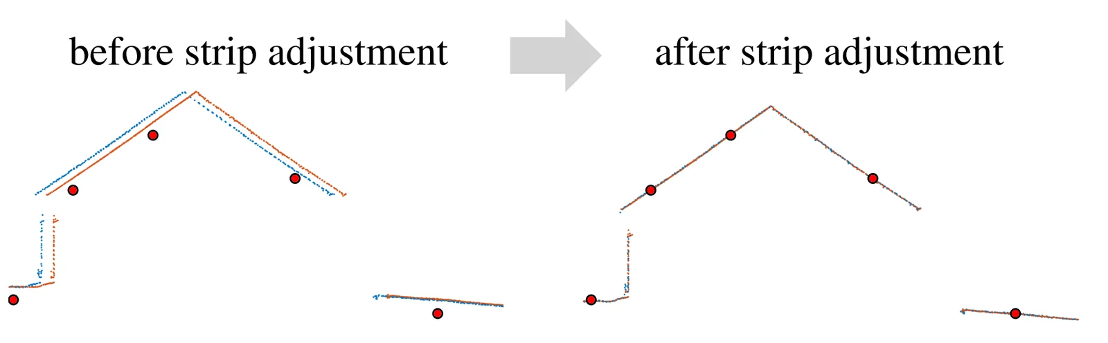
One roof profile, before and after strip alignment. Source: Glira et al. (2015), ISPRS Annals, CC BY 3.0.

Use the same roof before and after adjustment. Independent control checks absolute position.

4. Remove noise carefully

Some LiDAR returns do not represent the mapped surface. They can appear as isolated points or small clusters near terrain and vegetation [5].

First, flag obvious invalid points. Then compare each candidate with nearby terrain and objects. Jiang and colleagues tested this global-to-local approach on four airborne datasets [5].

A low point in a valley can be valid terrain. The same elevation can be an outlier in another location.

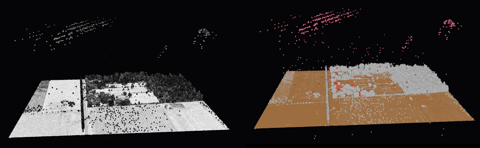
Two aligned views of the same airborne block: raw returns on the left, and on the right the same cloud with ground and vegetation classified and isolated high returns flagged. — Isolated returns above the surface, flagged as noise candidates beside the retained cloud.

Sparse objects need review too. A conductor may contain only a few points. Keep the noise decision reversible so a reviewer can restore real points.

5. Tile the point cloud

Large surveys may not fit in memory at once. Tiling divides the survey into smaller areas and supports neighborhood queries [2].

A hard tile edge can remove nearby context. A point near the edge may lose points that a surface normal or model feature needs.

Use a buffer around each tile. Process the buffer with the tile, then keep predictions from the tile core. That rule preserves local context without duplicating final points [2], [6].

Tile size also affects the result. Widyaningrum and colleagues found block effects with small blocks and lost detail with large blocks [6].

6. Prepare the model inputs

Feature preparation turns stored point records into model inputs. A model may use raw coordinates. It may also use height above ground or local geometric features [2], [8].

Production inputs must follow the same definitions and units used during training. The workflow also needs a clear rule for missing values.

A radius query selects points within a physical distance. A nearest-neighbor query selects a fixed point count. These queries describe different local areas [2].

Height normalization subtracts an estimated ground surface from each point elevation. Errors in that ground surface can create classification errors [7].

7. Run inference and keep the scores

The model receives prepared points and assigns a score to each allowed class. The highest score becomes the provisional label [8].

The label hides the other scores. Near an object boundary, two classes may have close scores. That shows a small model preference, not a probability of error [8].

Keep the raw scores with each tile. Record the model version and feature recipe too. Those records support later review.

Zhu and colleagues tested an encoder-decoder network on two datasets with different class schemas. Their results do not predict accuracy for an unrelated survey [8].

The next image shows one real tile as scores and provisional labels. Look for a boundary where two class scores sit close together.

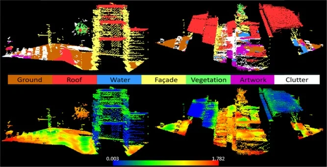
Aligned point-cloud views showing provisional semantic labels above a continuous per-point score field from the same inference run. — Provisional labels above, and the per-point score field behind them. Source: Lin et al. (2020), ISPRS Journal, CC BY 4.0.

The label map shows only the winning class. The score view shows how close that decision was. Rare classes need separate checks because overall accuracy can hide poor recall for a class with few points [9].

8. Reconcile repeated predictions

Buffered tiles can produce repeated predictions for one source point. Reconciliation chooses one final label [8].

The workflow can keep the core prediction or use a documented score rule. Zhu and colleagues used nearest-neighbor voting to merge repeated predictions and label omitted points [8].

Post-processing should solve a named error. Niemeyer and colleagues used nearby labels in an urban study. They later used morphological opening for building and tree products [7].

That study used urban data. Test every smoothing rule against reference data before applying it across a project.

9. Check geometry and labels

Geometric checks compare the cloud with independent control. Vertical residuals show elevation differences and can reveal local deformation [3], [10].

Large outliers can distort a mean. Höhle and Höhle recommend robust statistics when elevation errors do not follow a normal distribution [10].

Label checks compare predictions with an independent reference. A confusion matrix shows which classes the model mixed up. Precision measures correct predicted points. Recall measures recovered reference points [6].

The sample must represent the production project. Stehman and Czaplewski separate sample design from reference-label quality [11].

10. Export the classified cloud

The export step writes approved labels into the delivery schema. It should keep the required coordinate precision and source attributes [1], [2].

Record each changed field. LAS and LAZ can retain coordinates with extensible point attributes [1], [2].

Open the exported file as a new input. Compare its point count and bounds with the approved cloud.

11. Check the final products

Classified points can create a terrain model. They can also create a surface model or an object mask. Ground points support terrain interpolation. A canopy height model subtracts terrain elevation from a canopy surface [10], [12].

Each product has its own rules. A surface needs a cell size and interpolation method. An object mask needs a boundary rule.

Point-level checks do not prove that a final product meets its specification. Zhang and colleagues found that pits and smoothing choices changed estimated tree height [12].

The next image shows the classified source cloud beside products made from it. Use the same geographic extent in every panel.

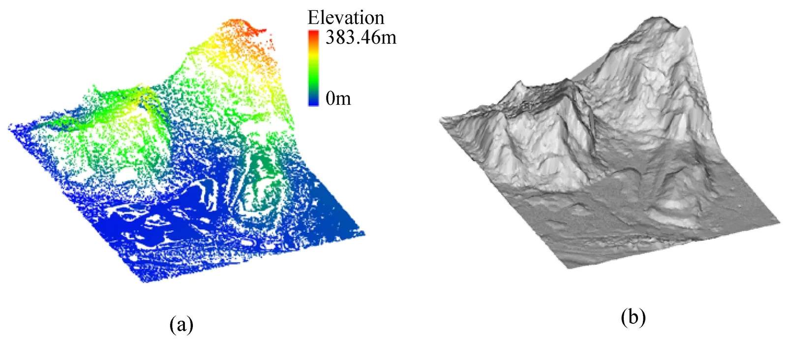
Two aligned panels over the same extent: ground points coloured by elevation, and the continuous terrain surface interpolated from them. — Ground points and the terrain surface derived from them. Source: Cai et al. (2019), Remote Sensing, CC BY 4.0.

The image makes the separate transformations visible. Check the final product at the scale and unit the user will use.

Conclusion

The model is one part of the workflow. It needs correct coordinates and aligned geometry. It also needs the input definitions used during training.

Check each step before the next one starts. Then check the final product, not only the point labels. This gives the team evidence that the delivery fits its intended use.

Vecten Desktop handles the classification and the review of the labels it produces, and it runs locally on your own workstation. The rest of the chain stays where it already is.

References

[1] M. Isenburg, "LASzip: Lossless compression of LiDAR data," *Photogrammetric Engineering & Remote Sensing*, vol. 79, no. 2, pp. 209-217, 2013, doi: 10.14358/PERS.79.2.209.
[2] J. Otepka, S. Ghuffar, C. Waldhauser, R. Hochreiter, and N. Pfeifer, "Georeferenced point clouds: A survey of features and point cloud management," *ISPRS International Journal of Geo-Information*, vol. 2, no. 4, pp. 1038-1065, 2013, doi: 10.3390/ijgi2041038.
[3] Y. Zhang and X. Shen, "Direct georeferencing of airborne LiDAR data in national coordinates," *ISPRS Journal of Photogrammetry and Remote Sensing*, vol. 84, pp. 43-51, 2013, doi: 10.1016/j.isprsjprs.2013.07.003.
[4] P. Glira, N. Pfeifer, C. Briese, and C. Ressl, "Rigorous strip adjustment of airborne laserscanning data based on the ICP algorithm," *ISPRS Annals*, vol. II-3/W5, pp. 73-80, 2015, doi: 10.5194/isprsannals-II-3-W5-73-2015.
[5] G. Jiang, D. D. Lichti, T. Yin, and W. Y. Yan, "A maximum entropy based outlier removal for airborne LiDAR point clouds," *IEEE JSTARS*, vol. 17, pp. 19130-19145, 2024, doi: 10.1109/JSTARS.2024.3478069.
[6] E. Widyaningrum, Q. Bai, M. K. Fajari, and R. C. Lindenbergh, "Airborne laser scanning point cloud classification using the DGCNN deep learning method," *Remote Sensing*, vol. 13, no. 5, art. no. 859, 2021, doi: 10.3390/rs13050859.
[7] J. Niemeyer, F. Rottensteiner, and U. Soergel, "Conditional random fields for LiDAR point cloud classification in complex urban areas," *ISPRS Annals*, vol. I-3, pp. 263-268, 2012, doi: 10.5194/isprsannals-I-3-263-2012.
[8] J. Zhu, L. Sui, Y. Zang, H. Zheng, W. Jiang, M. Zhong, and F. Ma, "Classification of airborne laser scanning point cloud using point-based convolutional neural network," *ISPRS International Journal of Geo-Information*, vol. 10, no. 7, art. no. 444, 2021, doi: 10.3390/ijgi10070444.
[9] X. Nong, W. Bai, and G. Liu, "Airborne LiDAR point cloud classification using PointNet++ network with full neighborhood features," *PLOS ONE*, vol. 18, no. 2, art. no. e0280346, 2023, doi: 10.1371/journal.pone.0280346.
[10] J. Höhle and M. Höhle, "Accuracy assessment of digital elevation models by means of robust statistical methods," *ISPRS Journal of Photogrammetry and Remote Sensing*, vol. 64, no. 4, pp. 398-406, 2009, doi: 10.1016/j.isprsjprs.2009.02.003.
[11] S. V. Stehman and R. L. Czaplewski, "Design and analysis for thematic map accuracy assessment: Fundamental principles," *Remote Sensing of Environment*, vol. 64, no. 3, pp. 331-344, 1998, doi: 10.1016/S0034-4257(98)00010-800010-8).
[12] W. Zhang, S. Cai, X. Liang, J. Shao, R. Hu, S. Yu, and G. Yan, "Cloth simulation-based construction of pit-free canopy height models from airborne LiDAR," *Forest Ecosystems*, vol. 7, art. no. 1, 2020, doi: 10.1186/s40663-019-0212-0.